Flow Analyzer

Flow Analyzer is a versatile tool that allows you to examine the details of what kind of traffic flows the total traffic is composed of.

1. Overview #

The Flow Analyzer in Scope, under the Flows tab, is a tool within a tool, displaying the individual traffic flows that make up the total captured traffic on the monitored interface, based on the given packet filter. It reveals which devices are communicating, where they are sending data, which protocols they use, and how much traffic they generate.

By adding classification rules, you can group them into easily managed categories and instantly spot new or unknown traffic. This adds a security dimension, allowing you to quickly detect any unauthorized or unexpected flows.

Additionally, the tool helps verify whether the packet filter is working as intended, which is particularly useful in complex measurement scenarios. With historical data at your fingertips, you no longer need to capture and analyze cumbersome full packet dumps to identify the flows behind an unexpected traffic spike.

The view has the following columns available:

Each flow has a state, which can have one of three values:

• New - The flow is new and reported for the first time
• Persistent - The flow is active or has been inactive less than the set limit
• Old - The flow has been inactive longer than the set limit and will be removed the next time flow results arrive

The inactivity counts duration from the last observed packet in the flow. If the flow is active, this number remains at or near zero. When a flow stops, i.e., no more packets are observed related to that, the inactivity begins to increase. Once it reaches the set limit, i.e., Flow timeout, the flow is deemed ended and will be removed from the visualization.

When saving flow information to a file, the format is a bit different, see Flow Results.

2. Startup #

Starting Flow Analyzer is very simple:

• Pick a measurement point from where you want to see the flows.
• Connect Probe in that measurement point by Scope.
  • If there is no Probe available yet, install it.
• Select the network interface where you expect the interesting traffic to be visible.
• What traffic are you interested in?
  • All the traffic destinated to or originating from the measurement point
    • Just start measuring.
  • All the traffic traversing the node
    • Set an empty filter as the manual packet filter and start measuring.
  • Only particular traffic
    • Set the packet filter according to your needs and start measuring.
• Now your measurement is running and you can move to the Flows tab, and observe the traffic flows in real-time.

3. Naming the Flows #

3.1. Ruling #

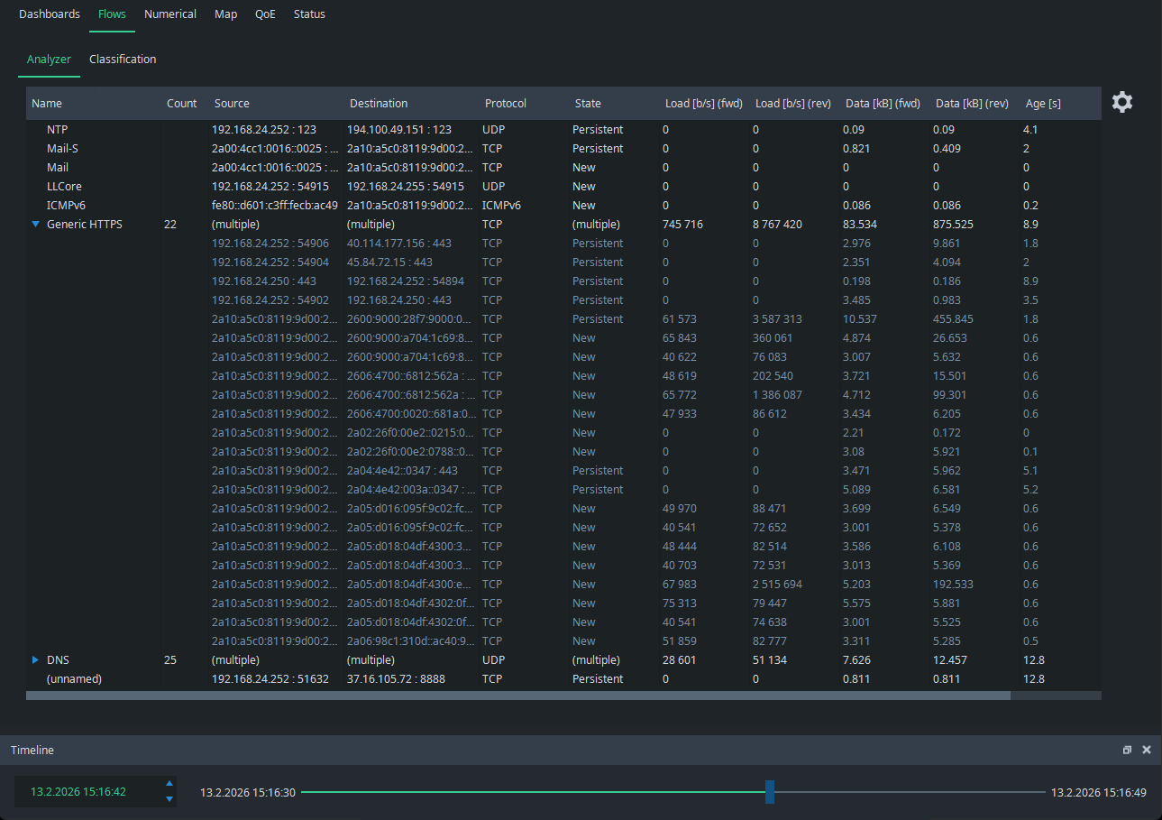
In the beginning, the flow view may look as follows:

As seen, all the flows appear as unknown. The reason is obvious: you have not yet named any flows, or at least the ones now showing. Go to Classification tab, and you find it empty:

This is the place where you define the classification rules for flows, e.g.,:

• General rule: a non-defined field means an asterisk
• All the fields with accurate addresses defined
  • Strict naming for only a single flow
• Only one address defined (either one)
  • All the flows containing the defined address will be categorized under this name.
• Only one port defined (either one)
  • All the flows containing the defined port will be categorized under this name.
• Both addresses defined
  • All the traffic between these two addresses will be categorized under this name.
• A protocol and one address defined
  • All the flows that contain the address and follow the defined protocol will be categorized under this name.
• A network defined (either one)
  • All the flows with either one of the IP addresses falling into this network will be categorized under this name.
  • Example: 192.168.0.0/24

Flows are classified for the first matching naming rule.

3.2. Classifying, by an Example #

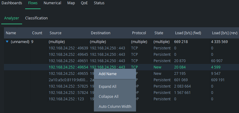
You can name the flows directly in the Classification tab, but let’s go back to the flow view because naming is more illustrative to start there. Pick a flow that you want to name and press the right mouse button on it. A menu appears: select Add Name. You can also double-click a flow row, which automatically moves you to the Classification tab with the flow information pre-filled.

The view returns to the Classification tab and the information of the selected flow appears as a new rule:

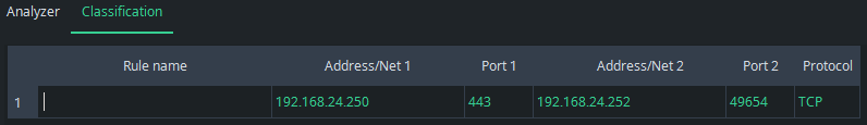
In this example, you know that the address 192.168.24.250 hosts a web-based factory control center using HTTPS (port 443). Thus, give an appropriate name and also remove the other address and port to include traffic from all sources to the control center under this rule. The final rule becomes then:

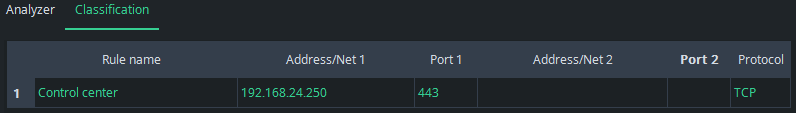
Go back to Analyzer to see the effect: the group of Control center appears with the flows that matched the rule:

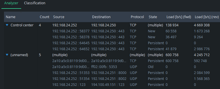
Use the blue triangle on the left side of the name to open and close the group:

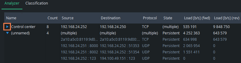
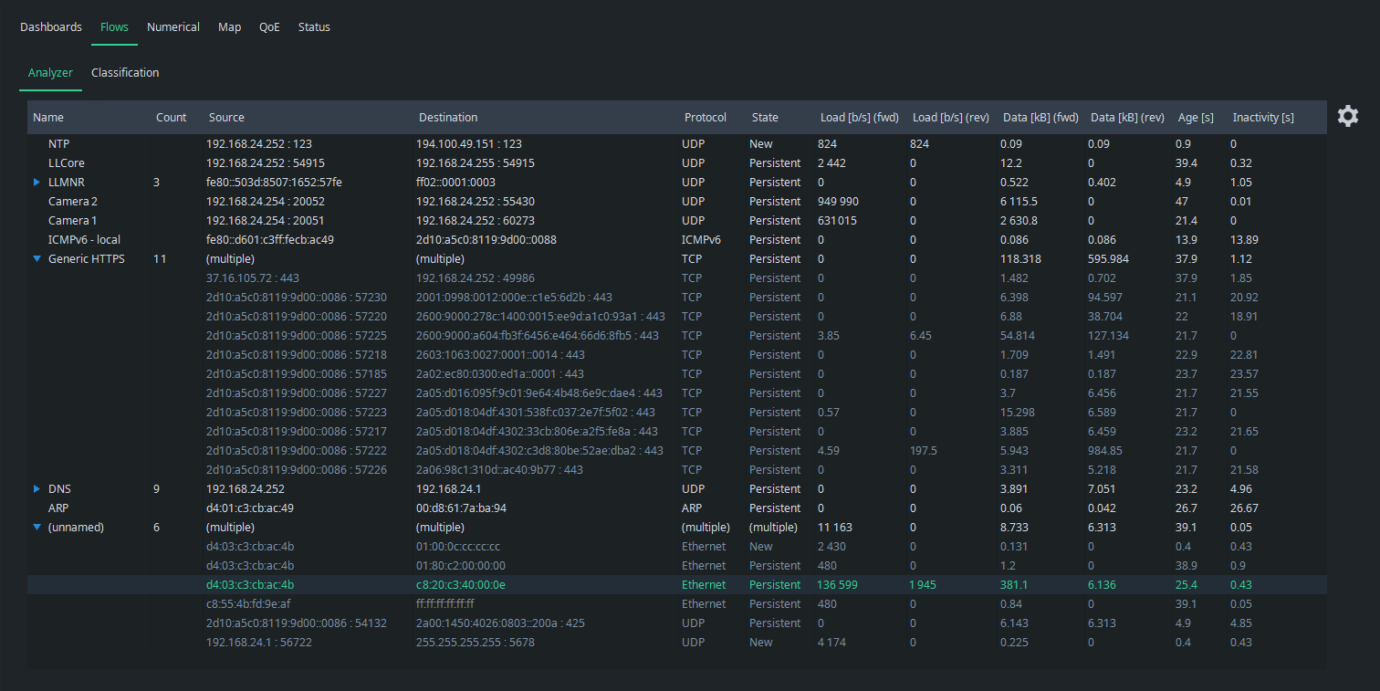
You also know that the UDP traffic with port 123 in both directions is caused by NTP. Then, IP address 192.168.24.251 is now an industry robot, and there are two cameras onboard using ports 8000 and 8002. Set rules also for these, and we get:

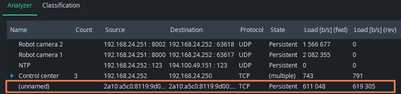
What started as an intricate list of some unknown flows, it all makes sense now. We see all the known flow categories clearly, but there still is one unknown flow. It seems to use IPv6 addressing and weird TCP ports (not shown in the picture). It has continuous traffic in both directions, now about 600 kbit/s. Perhaps it is a factory device we forgot, or has one of the applications or devices started to misbehave somehow? Or maybe it is traffic injected by malware! Whatever it is, it is now easy to check the originating device and the process there. This is one of the main points of flow analysis: know what is being transferred in your network.

3.3. Manipulating Rules #

By right-clicking your mouse over the Classification table, a menu appears where you can easily add new rules (Add Row) and delete them (Delete Row). You can also move the places of the rules.

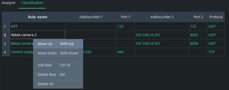
The order of the rules matters: if the rules overlap, i.e., a flow falls under multiple rules, the first one in the list will be picked. Consider the following rules:

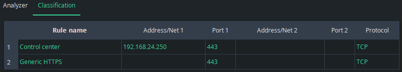
If there is HTTPS traffic from IP address 192.168.24.250, it will be categorized as Control center traffic despite fact that it also fits the second rule.

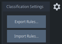
3.4. Storing and Loading Classification Lists #

Naturally, you don’t want to build the same classification rules over and over again each time you use Qosium Scope. Thus, click the gearwheel icon on the right to open Classification Settings. The button Export Rules saves the current classification rules. Import Rules loads the rules from a file. The corresponding configuration files are text files that you can also easily manipulate using an external text editor.

If you want to always use the same rule set, then you might want to save those as default. You can do this in the top menu bar: File => Defaults => Save Settings as Default. Bear in mind, however, that it will also save all the other settings you currently have in use.

Qosium Scope also carries a set of rules for known applications using particular transport layer protocols and ports. These classification rules lie in a file in the Scope’s binary directory named as well_known.ini.

4. Flow Analyzer Settings #

Flow Analyzer settings are available via the gearwheel icon on the right:

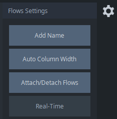
The available settings are:

• Add Name - An alternative way to add a flow name from the analyzer view
• Auto Column Width - Sets the width of the columns in the view automatically based on the content length.
• Attach/Detach Flows - Provides you a way to detach the analyzer view as a separate window and back.
• Real-Time - When browsing flow history, this button becomes active, letting you quickly get back to the real-time view.

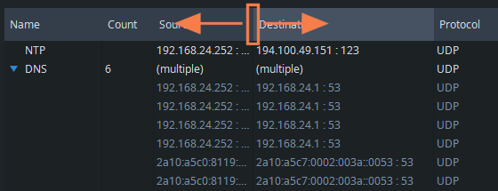
Column widths can also be adjusted manually. Just grab a side of a column header with your mouse and resize the width of the column according to your needs:

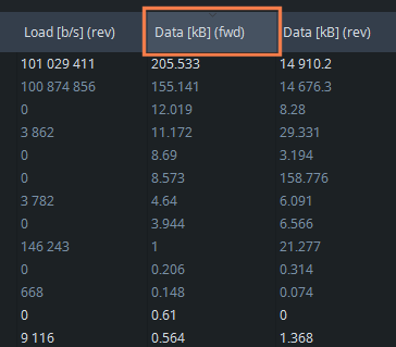
Flows in the analyzer view can be sorted by clicking the desired column header with a mouse. The default order is ascending. By clicking the same column header again, the order is reversed to descending. Please note that the categories are sorted first, and then the flows inside the categories. For example, to sort flows according to the transmitted data amount in descending order, click twice on the corresponding header:

5. Browsing Past Flow Information #

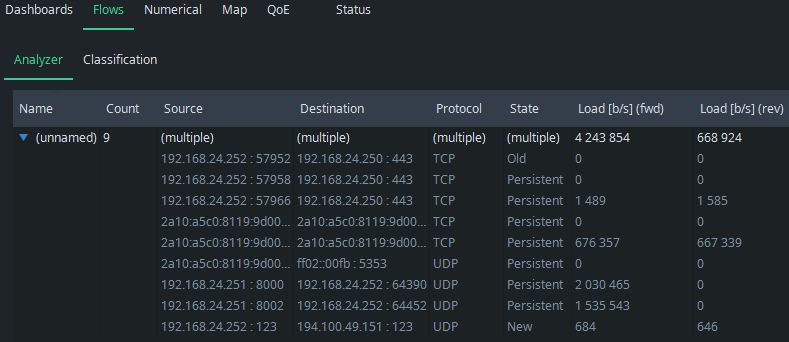
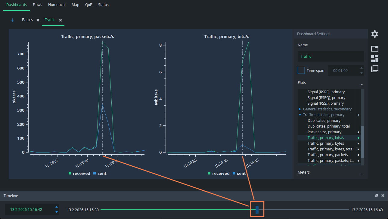
Imagine the following situation: you are performing a single point measurement and there is very little traffic. Suddenly, a higher traffic burst appears:

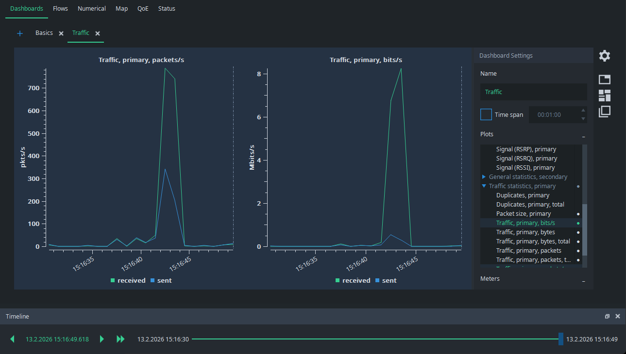
What caused that? Normally, you would need full packet captures to figure it out, but Qosium offers a considerably lighter way to do it. Grab the Timeline pointer and draw it back to the moment of the spike. You see the dashed line in the figures pointing to the place of the timeline:

Then, just go to the Flow Analyzer, and you see the flows that were active at that time. It is easy to see that the spike was caused by a set of HTTPS flows, most likely caused by downloading a web page with multiple media objects: